Friday, April 21, 2006
Wednesday, April 19, 2006
Figuring out E0
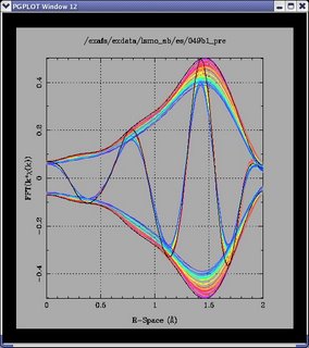
So to figure out what E0 is, we simply take the standard file and do a Fourier transform from k-space to r-space (using the same range of course) and plot it on top of a low temperature data file. You look at the zero crossings and then change the field "E0 shift in (eV)". Try 5.0eV and -5.0eV to get an idea of how to shift it. You can either shift the standard file, or the actual data file. Here's what I got:
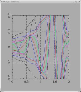
Ok so the black trace (hard to see) is the actual real data file. The red trace is the UNshifted standard file. The blue trace is -5.0eV shifted, the green trace is +5.0eV, the cyan trace is shifted +6.0eV, and the magenta trace is at +8.0eV.

Ok so the black trace (hard to see) is the actual real data file. The red trace is the UNshifted standard file. The blue trace is -5.0eV shifted, the green trace is +5.0eV, the cyan trace is shifted +6.0eV, and the magenta trace is at +8.0eV.
Tuesday, April 18, 2006
Start Fit #2

So the black trace is a sample trace of our lsmo sample in the ab-plane, and the red trace is the mn-o ab-plane standard file. I think they look reasonable, but I'll have to wait to see what Bud has to say.
ZOOM:

Ok so I looked up Travis' rsfit files and changed some stuff and ran it here's what I got:

ZOOM:


Friday, April 14, 2006
Travis is GOD
good standard from travis:
lsmo_mn_o_ab_1.9372.scf.4.f8
feff.inp file for c-axis: go up one lvl for ab plane:
/home/staff/tobrien/fit/structures/bilayer_lsmo/old/feff8/c
lsmo_mn_o_ab_1.9372.scf.4.f8
feff.inp file for c-axis: go up one lvl for ab plane:
/home/staff/tobrien/fit/structures/bilayer_lsmo/old/feff8/c
SSRL end of run form
Collecting good polarized EXAFS data on single crystal samples for both transmission and fluoresence is difficult because of Bragg diffraction from the sample, which changes the x-ray absorption in the sample. Usually one collects the data at a series of angles, and then combines the data to overcome this issue. For the bilayer CMR manganites we are studying, we have very thin oriented single crystals (mounted over a hole in a larger piece of the same single crystal material); however our first attempts to obtain transmission data (2+ years ago at the APS) failed because the Bragg spikes were too large.
Since then we have been using fluorescence data collection which is time consuming and has poorer data quality than for transmission. Last summer together with A. Mehta we showed on a diffraction beamline, that the problems in the transmission EXAFS were indeed caused by a number of Bragg diffractions; further we showed that oscillating the sample about vertical and horizontal axes, effectively averaged out the Bragg spikes if the oscillation angle was large enough (+- 2 deg) - we have now designed a wobbler to rotate the samples by a few degrees about horizontal and vertical axes (while the sample is in a He cryostat) and obtained the first good transmission data on one of the bilayer samples La(1.28)Sr(1.72)Mn2O7. Our preliminary data
reduction indicates consistent data. We also collected some fluorescence data using the same
method.
Thursday, April 13, 2006
Split them up
So now I need to break up the larger set into three smaller sets:
3K-50K: 049b1-2; 050b1;051b1-3;053b1-3
100K-124K: 056b1-3; 057b1-2; 058b1; 059b1; 060b1-2; 061b1-3; 062b1; 063b1-2
128K-160K: 065b1-3; 066b1-3; 067b1-3; 068b1-3; 069b1-3
180K-325K: 070b1-3; 071b1-4; 072b1-3; 0731-4; 074b1-3
Ok so after looking at all of these files we didn't really notice anything strange besides the fact that the peaks were shifting around atonically. Decided there's a background issue and went back to re-re-re-reduce the data.
I'm slowly varying the fourier transform range, the power of (E-E0), and the # of knots. Here's the two best settings so far:
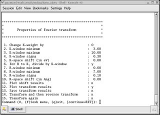
Above used a power of 1, and 6 knots with a window from 3 to 10:
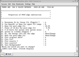
Above used a power of 0.5, and 5 knots with a window from 3 to 10:
3K-50K: 049b1-2; 050b1;051b1-3;053b1-3
100K-124K: 056b1-3; 057b1-2; 058b1; 059b1; 060b1-2; 061b1-3; 062b1; 063b1-2
128K-160K: 065b1-3; 066b1-3; 067b1-3; 068b1-3; 069b1-3
180K-325K: 070b1-3; 071b1-4; 072b1-3; 0731-4; 074b1-3
Ok so after looking at all of these files we didn't really notice anything strange besides the fact that the peaks were shifting around atonically. Decided there's a background issue and went back to re-re-re-reduce the data.
I'm slowly varying the fourier transform range, the power of (E-E0), and the # of knots. Here's the two best settings so far:

Above used a power of 1, and 6 knots with a window from 3 to 10:

Above used a power of 0.5, and 5 knots with a window from 3 to 10:
Re-re-Reduce
So came in today and tweeked up the pre-edge and background removal. I moved the "start XXXeV above edge" parameter to 170eV. It was at ~150eV and looked like it was falling on the top of a peak. I also pushed the low end of the fit range up a little bit, also looked like it was coming in on a peak. Then I just Fourier transformed it and got this:
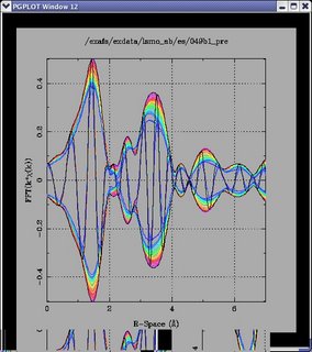
In K-space:

In R-space:
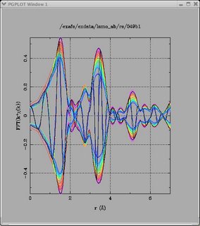
It looks to me like I got rid of the shoulder problem. I still need to check Lisa's suggestion for the outlyer (06xb-whatever), which is that E-E0 is varying.
In K-space:

In R-space:

It looks to me like I got rid of the shoulder problem. I still need to check Lisa's suggestion for the outlyer (06xb-whatever), which is that E-E0 is varying.
Wednesday, April 12, 2006
Reducing AB-plane data
So all of the earlier stuff was from the c-axis data:
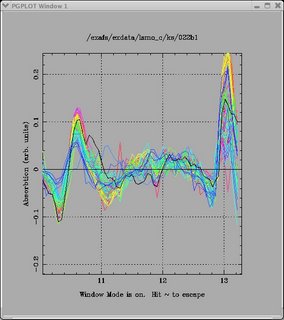
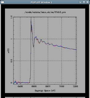
Here's the normalized plot in energy space of the ab-plane data:
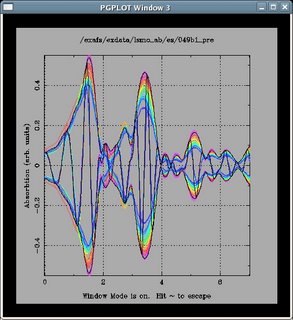
Things get kinda funky in k-space. Here's the plot:
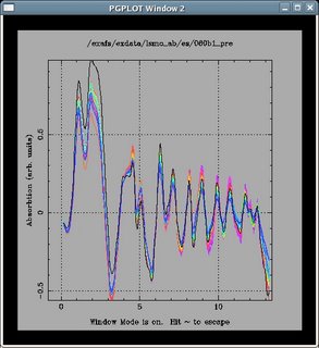
Notice the black highlighted outlying trace. That's 060b1:
Here's is the real space data:
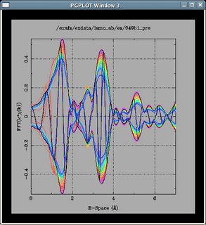
And here's the real space data post- y2 correction:
Guess what that red- low r outlier is...060b1- who would've thought?
Here's the normalized plot in energy space of the ab-plane data:

Things get kinda funky in k-space. Here's the plot:

Notice the black highlighted outlying trace. That's 060b1:
Here's is the real space data:

And here's the real space data post- y2 correction:

Guess what that red- low r outlier is...060b1- who would've thought?
Reducing AB-plane data
So all of the earlier stuff was from the c-axis data:
Here's the normalized plot in energy space of the ab-plane data:

Things get kinda funky in k-space. Here's the plot:

Notice the black highlighted outlying trace. That's 060b1:
Here's is the real space data:

And here's the real space data post- y2 correction:

Guess what that red- low r outlier is...060b1- who would've thought?
Here's the normalized plot in energy space of the ab-plane data:

Things get kinda funky in k-space. Here's the plot:

Notice the black highlighted outlying trace. That's 060b1:
Here's is the real space data:

And here's the real space data post- y2 correction:

Guess what that red- low r outlier is...060b1- who would've thought?
Tuesday, April 11, 2006
Start Fit
Ok so now I need to begin fitting the data. We use a program called RSFIT. It works pretty good: here's what I've got so far. Here's my input file:

And here's what it looks like plotted with the actual data (data is in red):

Not the best...the phase is off...why is that? And the peak of the fit is a little bit low.

And here's what it looks like plotted with the actual data (data is in red):

Not the best...the phase is off...why is that? And the peak of the fit is a little bit low.
Monday, April 10, 2006
Not sure of the glitch...
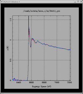
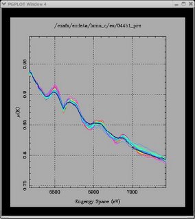
We re-did the pre edge using 185eV above the edge for our background removal.
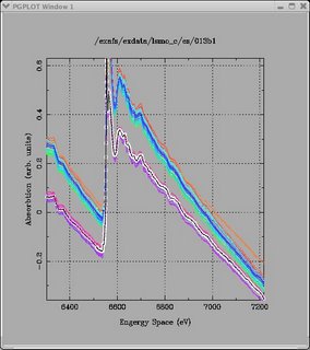
Here's the new normalized post pre-edge removal spectra:
And the zoom:
Now I need to re-do the k-space data and the r-space data and see how it turns out.
I'm going to leave the last bit of data out with the crazy up turn at the end:
use k_max = 12.6 and fft k_max of 12.1;
K-space plot:
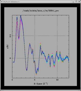
Here's what I got:
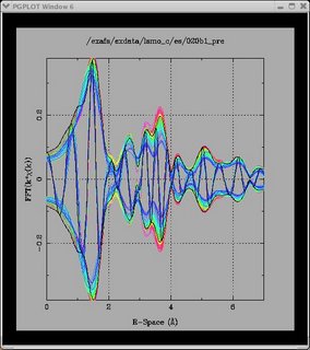
Now you can see that I've gotten rid of that horrible shoulder problem, and most (~80%) of the traces don't have the "wiggle" problem either, this one which happens to be the first data set, is the worst by far:
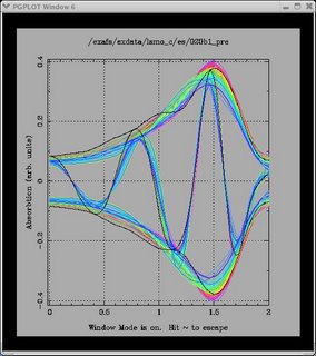
Here's the new normalized post pre-edge removal spectra:

And the zoom:

Now I need to re-do the k-space data and the r-space data and see how it turns out.
I'm going to leave the last bit of data out with the crazy up turn at the end:
use k_max = 12.6 and fft k_max of 12.1;
K-space plot:

Here's what I got:

Now you can see that I've gotten rid of that horrible shoulder problem, and most (~80%) of the traces don't have the "wiggle" problem either, this one which happens to be the first data set, is the worst by far:

Weird Shoulders
028b1
029b1-2
030b1-3 (b2 is ok...)
031b1-3
032b1-3
Above has weird shoulders around 1.2-1.3A. Here's a plot (the highlighted trace is in black):

-------------
022b1
023b1
023b2
024b1
042b1
Above doesn't have shoulders- but had weird dips in the less than 1.2A area. Here's a plot:

---------
039b3
043b1
043b2
044b1
Above has a flatened top, and in some cases looks like two peaks. Here's a plot:

029b1-2
030b1-3 (b2 is ok...)
031b1-3
032b1-3
Above has weird shoulders around 1.2-1.3A. Here's a plot (the highlighted trace is in black):

-------------
022b1
023b1
023b2
024b1
042b1
Above doesn't have shoulders- but had weird dips in the less than 1.2A area. Here's a plot:

---------
039b3
043b1
043b2
044b1
Above has a flatened top, and in some cases looks like two peaks. Here's a plot:

Reduce Numero Tres
This is the E-space file that has been normalized and pre-edged.

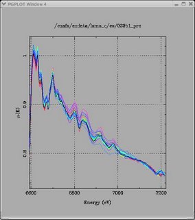
So, in this next plot is just a blown up view of the middle section of the energy space file. You can see how the different traces seperate? That's bad!
This is the real space plot of the lsmo c-axis data. See the shoulder below ~1.2A. That can't be there since an atom is only ~1A or maybe even a little bit more. We think that the pre-edge was not done corretly and I want to check to see if it is correct or not.

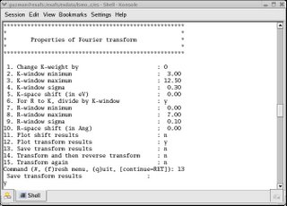
And finally this is my input parameters into the Fourier transform from K-space to real space.

So, in this next plot is just a blown up view of the middle section of the energy space file. You can see how the different traces seperate? That's bad!

This is the real space plot of the lsmo c-axis data. See the shoulder below ~1.2A. That can't be there since an atom is only ~1A or maybe even a little bit more. We think that the pre-edge was not done corretly and I want to check to see if it is correct or not.

And finally this is my input parameters into the Fourier transform from K-space to real space.

Thursday, April 06, 2006
Reduced Woes Part 2
Ok so I made a little more progress tonight:
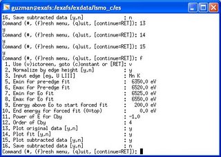
I decided to just try to do the pre edge without worring about the normalization, using [ret] mode, and got it to work so I was encouraged. Next, I tried victoreen mode and got that to work out as well. Then when I tried normalizing to edge height, I got the blank file again. so I'm definately doing that wrong. Here is my best pre-edge graph and my comdata file.


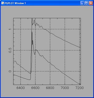
The red plot is the original data, and the black plot is the "pre-edge reduced" data (of course its not really since its wrong!)
I decided to just try to do the pre edge without worring about the normalization, using [ret] mode, and got it to work so I was encouraged. Next, I tried victoreen mode and got that to work out as well. Then when I tried normalizing to edge height, I got the blank file again. so I'm definately doing that wrong. Here is my best pre-edge graph and my comdata file.


The red plot is the original data, and the black plot is the "pre-edge reduced" data (of course its not really since its wrong!)
Wednesday, April 05, 2006
Wobbler Pictures

This is a picture of the center oscillator, which rotates the sample horizontally about the vertical axis. The pivots are connected to the sample holder vertically.
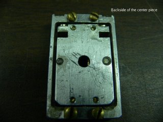
This is the back side of the center oscillator. You can see the two magnets which are epoxied in place. The stack of magnets which moves in and out of the driving coil are held in place by these small magnets.

This is a view of the fully assembled oscillator connected to the cryostat probe. The sample is also mounted and held in place by a springy metal, I belive copper-berilium- need to check this: if you could comment on this Bud. This is the front end. One major improvement needs to be in how the wires are held in place. This grey terminal block is too large, and the connectors we were using are too large.

This is the back side of the oscillator connected to the probe. This is where the most improvement needs to be. Having the two coils (one driving- one pickup) horizontally in line created some issue with the cryostat. They would get pushed in by the sides of the cryostat and would then become misaligned. They need to be smaller and more robust.

